Running Workflows
Introduction
Once you have a working installation of atomate2, you’ll want to jump in and start running workflows. Atomate2 includes many workflows with reasonable settings that can get you started. This tutorial will quickly guide you through customizing and running a workflow to calculate the band structure of MgO.
Objectives
Run an atomate2 workflow using Python
Analyze the results using pymatgen
Prerequisites
For you to complete this tutorial you need
A working installation of atomate2.
Bandstructure Workflows
A fundamental and common use of DFT is to calculate band structures and electronic densities of states. Here we will use an atomate2 workflow to calculate the bandstructure of MgO. The workflow consists of 4 parts:
A structural optimisation.
A self-consistent static calculation on the relaxed geometry.
A non-self-consistent calculation on a uniform k-point mesh (for the density of states).
A non-self-consistent calculation on a high symmetry k-point path (for the line mode band structure).
Running a Bandstructure Workflow
Setup
Make sure you have completed the installation tutorial. Next, create a folder on your HPC resource for this tutorial. It can be located anywhere that you can submit and run jobs. You’ll keep all of the files for this tutorial there.
Create the workflow in Python
Workflows in atomate2 are composed of two objects:
Jobs: A single unit of computation. Roughly speaking, each
jobcorresponds to one VASP calculation.Flows: A collection of
jobsconnected together. The band structure workflow we are running is an example of aflow.Flowscan be nested, for example, you could have multiple band structureflowsin a single workflow.
A list of all VASP workflows (which covers both jobs and flows) is given in the
List of VASP workflows section of the documentation. Workflows are created
using Maker objects. These return the workflows that can be executed later.
In this example, we will use the RelaxBandStructureMaker to construct our
workflow.
Create a Python script named mgo_bandstructure.py with the following contents:
from atomate2.vasp.flows.core import RelaxBandStructureMaker
from jobflow import run_locally
from pymatgen.core import Structure

# construct a rock salt MgO structure
mgo_structure = Structure(
    lattice=[[0, 2.13, 2.13], [2.13, 0, 2.13], [2.13, 2.13, 0]],
    species=["Mg", "O"],
    coords=[[0, 0, 0], [0.5, 0.5, 0.5]],
)

# make a band structure flow to optimise the structure and obtain the band structure
bandstructure_flow = RelaxBandStructureMaker().make(mgo_structure)

# run the job
run_locally(bandstructure_flow, create_folders=True)
Running the workflow
Similar, to the installation tutorial, now create a job script to execute the workflow.
Write your job script to the job.sh file. For example, on the Grid Engine queue
system, your job script would look something like:
#!/bin/bash -l
#$ -N relax_si
#$ -P my_project
#$ -l h_rt=1:00:00
#$ -l mem=4G
#$ -pe mpi 16
#$ -cwd

# ensure you load the modules to run VASP, e.g., module load vasp

conda activate atomate2
python mgo_bandstructure.py
Finally, submit the job to the queue using the normal scheduler command. For example
on the Grid Engine scheduler, this would be using qsub job.sh.
Once the job is finished, you can check that the workflow completed successfully by checking the standard output and error files produced by the job script.
Provided there weren’t any errors, the workflow has successfully finished and the results will be in your database.
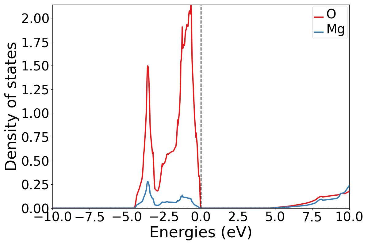
Analyzing a Bandstructure Workflow
Finally, we’ll plot the results that we calculated. Simply run the following Python code, either as a script or on the Python prompt.
from jobflow import SETTINGS
from pymatgen.electronic_structure.plotter import DosPlotter, BSPlotter
from pymatgen.electronic_structure.dos import CompleteDos
from pymatgen.electronic_structure.bandstructure import BandStructureSymmLine
store = SETTINGS.JOB_STORE
store.connect()
# get the uniform bandstructure from the database
result = store.query_one(
{"output.task_label": "non-scf uniform"},
properties=["output.vasp_objects.dos"],
load=True, # DOS stored in the data store, so we need to explicitly load it
)
dos = CompleteDos.from_dict(result["output"]["vasp_objects"]["dos"])
# plot the DOS
dos_plotter = DosPlotter()
dos_plotter.add_dos_dict(dos.get_element_dos())
dos_plotter.save_plot("MgO-dos.pdf", xlim=(-10, 10))
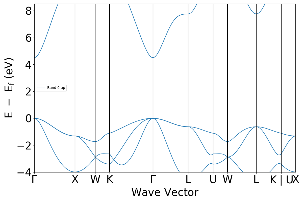
# get the line mode bandstructure from the database
result = store.query_one(
{"output.task_label": "non-scf line"},
properties=["output.vasp_objects.bandstructure"],
load=True, # BS stored in the data store, so we need to explicitly load it
)
bandstructure = BandStructureSymmLine.from_dict(
result["output"]["vasp_objects"]["bandstructure"]
)
# plot the line mode band structure
bs_plotter = BSPlotter(bandstructure)
bs_plotter.save_plot("MgO-bandstructure.pdf")
If you open the saved figures, you should see a plot of your DOS and bandstructure!
Conclusion
In this tutorial, you learned how to run a band structure workflow and plot the outputs.
To see what workflows can be run, see the List of VASP workflows. They can be set up and run in the same way as in this tutorial.
At this point, you might:
Learn how to chain workflows together: Chaining workflows.
Learn how to customise VASP input settings: Modifying input sets.
Learn more about Document Models and Schemas
Configure atomate2 with FireWorks to manage and execute many workflows at once: Using atomate2 with FireWorks.