Shockley-Read-Hall Recombination

Shockley-Read-Hall (SRH) recombination is the dominant recombination mechanism at lower carrier concentrations. First-principles calculations of the SRH recombination rate were pioneered in the Van de Walle group at the University of California, Santa Barbara by Prof. Audrius Alisauskas [Alkauskas et al., 2014]. Additional developments have been made to better integrate the methodology with existing projector-augmented wave methods in VASP to enable much faster calculations of the SRH recombination rate. For a more detailed account of the methodology, please see the following reference: [Shen, 2018].

# disable warnings
import warnings
warnings.filterwarnings("ignore", category=UserWarning)
from pathlib import Path
import numpy as np
from matplotlib import pyplot as plt
from pymatgen.analysis.defects.ccd import HarmonicDefect, get_SRH_coefficient

TEST_FILES = Path("../../../tests/test_files/v_Ga/")

Read a single Harmonic Defect

We can parse an sorted list of directories with HarmonicDefect.from_directories. This will look into each directory for a vasprun.xml file from which the structures and energies will be extracted.

The different constructors for HarmonicDefect all accept a list of sources where the energies and structures come from. The relaxed structure will be taken from the relaxed_index entry from this list and the electronic structure from this entry will be parsed to help identify the defect band in the band structure.

dirs01 = [TEST_FILES / "ccd_0_-1" / str(i) for i in [0, 1, 2]]
hd0 = HarmonicDefect.from_directories(
    directories=dirs01,
    store_bandstructure=True,
)
print(f"The relaxed structure is in dirs01[{hd0.relaxed_index}]")
print(hd0)
print(
    f"The spin channel ({hd0.spin}) is also automaticalliy determined by the "
    "IPR, by taking the spin channel who's defect states have the lowest average IPR across the different k-points."
)

The relaxed structure is in dirs01[1]
HarmonicDefect(omega=0.033 eV, charge=0.0, relaxed_index=1, spin=1, defect_band=[(138, 0, 1), (138, 1, 1)])
The spin channel (-1) is also automaticalliy determined by the IPR, by taking the spin channel who's defect states have the lowest average IPR across the different k-points.

Note that HarmonicDefect.defect_band consists of multiple states presented as (iband, ikpt, ispin) index tuples, if defect_band was not provided to the constructor, the relaxed_index entry in the directory list will be checked for a Procar file, which will be parsed to give the “best guess” of the defect state in the band structure. The band index is automatically determined by the inverse participation ratio. Note that the defect state reports the “most-localized” bands at each k-point so it is possible for the band index of the defect band to change for different kpoint indices ikpt.

Note: The automated defect state identification is still in testing you can provide the `defect_band` manually to over-ride the automatic behavior if you notice any issues. Please report any issues you encounter to the github issue tracker.

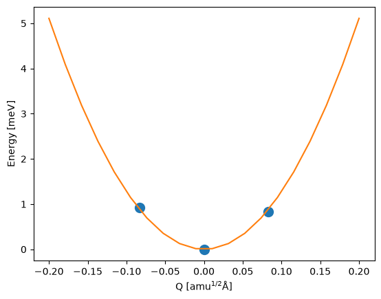
Potential energy surface

Under the harmonic approximation, the potential energy surface of the defect in a particular charge state is given by:

\[\frac{1}{2} \omega^2 Q^2\]

where \(\omega\) is the harmonic frequency and \(Q\) is the mass-weighted displacement (configuration coordinate) of the defect as it changes between different charge states.

plt.plot(
    hd0.distortions,
    (np.array(hd0.energies) - hd0.energies[hd0.relaxed_index]) * 1000,
    "o",
    ms=10,
)
xx = np.linspace(-0.2, 0.2, 20)
yy = 0.5 * hd0.omega**2 * xx**2
plt.plot(xx, yy * 1000)
plt.xlabel("Q [amu$^{1/2}$Å]")
plt.ylabel("Energy [meV]");

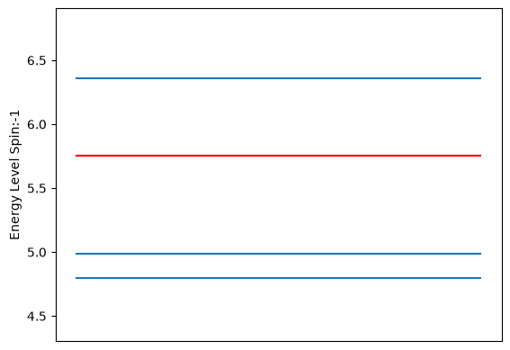
The band structure of the relaxed structure has a state that can be identified as the defect state using the inverse participation ratio.

bs = hd0.relaxed_bandstructure
eigs = bs.bands[hd0.spin][:, 1]
eigs_ref_efermi = eigs
plt.hlines([eigs_ref_efermi], 0, 1)
plt.hlines(eigs_ref_efermi[hd0.defect_band_index], 0, 1, colors="red")
plt.ylim(bs.efermi - 0.1, bs.efermi + 2.5)
plt.xticks([])
plt.ylabel(f"Energy Level Spin:{hd0.spin}");

Evaluating the Electron-Phonon Matrix Element with PAWs

Methods for evaluating electron-phonon interactions in solids from ab initio calculations are well established. We use the frozen-phonon method, whereby all the atoms in a supercell are displaced according to the eigenmode of the special phonon. The coupling between the atomic displacements and the electronic properties of the system is represented by the electron-phonon matrix element (epME). The epME of the special phonon (parameterized by Q) is given by:

\[ W_{if} = \left< \psi_i \left| \frac{\partial \hat h}{\partial Q} \right| \psi_f \right> = (\varepsilon_i - \varepsilon_f) \frac{\left<\psi_f | \psi_i({\delta Q}) \right>}{\delta Q}\]

Note that the initial and final states here are determined by the process you are studying. If you are looking at defect capture, the initial state will be the band edge state and the final state will be the defect state. The overlap above is for the all-electron wavefunction, under the PAW formalism in VASP the overlap in the expression above can be expressed using the psuedo-wavefunctions \(\tilde \psi_{i,f}\) and the overlap operator \(\hat S\):

\[ W_{if} = (\varepsilon_i - \varepsilon_f) \frac{\left<\tilde \psi_f |\hat S |\tilde \psi_i({\delta Q}) \right>}{\delta Q}\]

This expression above can be calculated with VASP version 6.0 and above by copying the WAVECAR file from the displaced (δQ) structure into the directory that already contains the relaxed calculations directory as WAVECAR.QQQ and then running VASP with LWSWQ = .TRUE.. This will calculate the overlap part in the expression above and write it into the WSWQ file. Automatic parsing of the WSWQ file has been implmented in pymatgen.io.vasp.outputs. The HarmonicDefect.get_elph_me method will read a list of WSWQ objects and compute the epME via finite difference by calculating the overlap for a series of displacements.

To compute the electron-phonon matrix element, we must first populate the wswq attribute of the HarmonicDefect object by reading the WSWQ files from a directory where they have been labeled in WSWQ.i where the index i is used to sort the WSWQ files to help compute the epME via finite difference. As an example, we will use the three WSWQ files generated by the three displaces in hd0

wswq_dir = TEST_FILES / "ccd_0_-1" / "wswqs"
print(f"The parsed WSWQ files are: {[f.name for f in wswq_dir.glob('WSWQ*')]}")
hd0.read_wswqs(TEST_FILES / "ccd_0_-1" / "wswqs")
print(f"Parsed {len(hd0.wswqs)} WSWQ files.")

The parsed WSWQ files are: ['WSWQ.0', 'WSWQ.1', 'WSWQ.2']

Parsed 3 WSWQ files.

The epME is computed by the HarmonicDefect.get_elph_me method, which requires the defect band index. Since we know the band edge state is at the Gamma point from analyzing the bulk cell and that the second kpoint index is Gamma in our supercell calculations, can pass the ikpt = 1 defect electronic state into the get_elph_me method.

print(f"The automatically determined defect electronic states are: {hd0.defect_band} "
    "(with [band, k-point, spin] indexing).")
epME = hd0.get_elph_me(defect_state=(138, 1, 1))
print(f"The resulting array of shape {epME.shape} contains the matrix elements from the "
    "defect state to all other states at the same k-point.")

The automatically determined defect electronic states are: [(138, 0, 1), (138, 1, 1)] (with [band, k-point, spin] indexing).
The resulting array of shape (216,) contains the matrix elements from the defect state to all other states at the same k-point.

Calculating the SRH Capture Coefficient

To calculate the Shockley-Read-Hall (SRH) capture coefficient, we also need the potential energy surface of the final state.

dirs10 = [TEST_FILES / "ccd_-1_0" / str(i) for i in [0, 1, 2]]
hd1 = HarmonicDefect.from_directories(
    directories=dirs10,
    store_bandstructure=True,
)

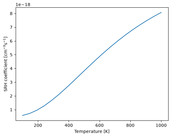
With the initial and final potential energy surfaces, and the WSWQ data for the initial state, we can calculate the SRH capture coefficient using the get_SRH_coefficient function to compute the capture coefficient as a function of temperature.

T = np.linspace(100, 1000, 20)
srh_c = get_SRH_coefficient(initial_state=hd0, final_state=hd1, defect_state=(138, 1, 1), T=T, dE=0.3)
plt.plot(T, srh_c)
plt.xlabel("Temperature [K]")
plt.ylabel("SRH coefficient [cm$^{-3}$s$^{-1}$]");