Formation Energy Diagrams

The formation energy diagram is perhaps the most important tool in analyzing the defect properties. It informs both the likelihood of a defect forming and the transition level where the charge state of the defect changes.

The formation energy of a defect is determined by the chemical potential of everything that goes into forming the defect. While all of the different chemical potentials are interconnected, it is conceptually easier to separate them into two groups: the chemical potential of the elements and the chemical potential of the electron. The chemical potential of the electron often called the Fermi level, accounts for how all of the external conditions, including the presence of other defects, affect the thermodynamics of adding or removing an electron from the defect. Since the electrons in the system can be manipulated after the defect is formed, the Fermi level is often considered a free variable and is shown as the x-axis in the formation energy diagram. The chemical potentials of the different atoms added or removed to form the defect are less dynamic and assumed to be fixed after the defect is formed.

The expression for the formation energy of a defect is given by:

\[E^f[X^q] = E_{\rm tot}[X^q] - E_{\rm tot}[{\rm bulk}] + \sum_i n_i \mu_i + qE_{\rm F} + \Delta^q \, ,\]

where \(E^f[X^q]\) is the formation energy of the defect, \(E_{\rm tot}[X^q]\) is the total energy of the defect, \(E_{\rm tot}[{\rm bulk}]\) is the total energy of the bulk, \(n_i\) is the number of atoms of type \(i\) in the defect, \(\mu_i\) is the chemical potential of atom type \(i\), \(q\) is the charge of the defect, \(E_{\rm F}\) is the Fermi level, and \(\Delta^q\) is finite-size correction which we have to add to account for image effects of simulating the defect in a periodic simulation cell.

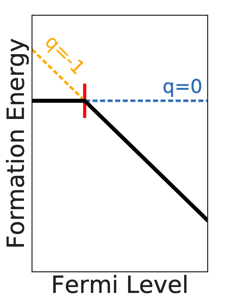
A schematic of the formation energy diagram for the \(q=0\) and \(q=-1\) charge states of a hypothetical defect is shown below.

Defining a Formation Energy Diagram

The class responsible for analyzing the formation energy is described by the following fields.

FormationEnergyDiagram(
    bulk_entry: 'ComputedStructureEntry',
    defect_entries: 'List[DefectEntry]',
    pd_entries: 'list[ComputedEntry]',
    vbm: 'float',
    band_gap: 'Optional[float]' = None,
    inc_inf_values: 'bool' = False,
)

Note: For now, the bulk entry and all the defect entries need to have the exact same supercell shape.

import warnings
from monty.serialization import loadfn
from pymatgen.analysis.defects.thermo import FormationEnergyDiagram
from pymatgen.io.vasp import Vasprun

warnings.filterwarnings("ignore")

from pathlib import Path

from pymatgen.analysis.defects.core import Substitution
from pymatgen.core import PeriodicSite, Species, Structure

TEST_FILES = Path("../../../tests/test_files")

gan_struct = Structure.from_file(TEST_FILES / "GaN.vasp")
# make a substitution site
ga_site = gan_struct[0]
mg_site = PeriodicSite(
    species=Species("Mg"), coords=ga_site.frac_coords, lattice=gan_struct.lattice
)
# instantiate the defect object
mg_ga = Substitution(structure=gan_struct, site=mg_site)

sc_dir = TEST_FILES / "Mg_Ga"
# ents = MPRester().get_entries_in_chemsys("Mg-Ga-N") # Query from MPRester
ents = loadfn(TEST_FILES / "Ga_Mg_N.json")  # Load from local
fed = FormationEnergyDiagram.with_directories(
    directory_map={
        "bulk": sc_dir / "bulk_sc",
        0: sc_dir / "q=0",
        -1: sc_dir / "q=-1",
        1: sc_dir / "q=1",
    },
    defect=mg_ga,
    pd_entries=ents,
    dielectric=10,
)

Getting the Elemental Chemical Potentials

All of the chemical potentials are, in principle, free variables that indicate the conditions of the surrounding environment while the defect is formed. These free variables are bound by the enthalpies of formation of the various compounds that share the same elements as the defect and bulk material. These competing compounds essentially establish the boundaries of the allowed chemical potentials, while the VBM and CBM of the bulk material determine the allowed range of the Fermi level. As such, first-principles calculations can be used to determine the limits of the various chemical potentials. As an example, the elemental chemical potentials for the Mg\(_{\rm Ga}\) defect in GaN are shown below:

\[\begin{split} \begin{aligned} \Delta\mu_{\rm Ga} + \Delta\mu_{\rm N} &= \Delta H_{\rm GaN} \\ 5\Delta\mu_{\rm Mg} + 2\Delta\mu_{\rm Ga} + \Delta\mu_{\rm N} &\leq \Delta H_{\rm Mg_5Ga_2} \\ 3\Delta\mu_{\rm Mg} + 2\Delta\mu_{\rm N} &\leq \Delta H_{\rm Mg_3N_2} \\ \end{aligned} \end{split}\]

Here since the defect must form in GaN the chemical potentials are pinned by the plane defined by the enthalpy of formation of GaN. The limits imposed by the competing compounds are shown by the additional inequalities. The points of interest are usually vertex points in the constrained chemical potential space so we report the full set of vertex points in FormationEnergyDiagram.chempot_limits.

for i, p in enumerate(fed.chempot_limits):
    print(f"Limits for the chemical potential changes for point {i}")
    for k,v in p.items():
        print(f"Δμ_{k} = {v:.2f} eV")

Limits for the chemical potential changes for point 0
Δμ_Mg = -1.49 eV
Δμ_Ga = -1.75 eV
Δμ_N = 0.00 eV
Limits for the chemical potential changes for point 1
Δμ_Mg = -0.35 eV
Δμ_Ga = -0.03 eV
Δμ_N = -1.71 eV
Limits for the chemical potential changes for point 2
Δμ_Mg = -0.44 eV
Δμ_Ga = 0.00 eV
Δμ_N = -1.75 eV

Finite-size corrections

Finite-size corrections are necessary to account for the fact that we are simulating a charged defect in a periodic simulation cell. The standard approach was developed by Freysoldt and co-workers and is described in the following paper:

[Freysoldt et al., 2009].

Freysoldt, C., Neugebauer, J., & Van de Walle, C. G. (2009). Fully Ab Initio Finite-Size Corrections for Charged-Defect Supercell Calculations. Phys Rev Lett, 102(1), 016402. doi: 10.1103/PhysRevLett.102.016402

This method requires calculating the the long range term from the Coulomb interaction and a short range term from the electrostatic potential in the LOCPOT file. While the final result of the finite-size correction is just a single number \(\Delta^q\) for each charge state, the intermediate results can still be analyzed. This is still useful, since the defect position is automatically determined from the LOCPOT files alone, to check the planar-averaged potential plots to make sure that the defect is indeed in the correct position. This will be evident if the planar-averaged potential difference is peaked at the two ends of the plot since the automatically determined defect position is chosen as the origin of the plot. The short range contribution is set to zero far away from the defect, which is accomplished by average the planar electrostatic potential far away from the defect in the sampling region shown below. The intermediate analysis (planar-averaged potentials) for calculating the Freysoldt correction for each of the the three lattice directions is shown below.

from pymatgen.analysis.defects.corrections.freysoldt import plot_plnr_avg
plot_data = fed.defect_entries[1].corrections_metadata["freysoldt"]["plot_data"]
plot_plnr_avg(plot_data[0], title="Lattice Direction 1")
plot_plnr_avg(plot_data[1], title="Lattice Direction 2")
plot_plnr_avg(plot_data[2], title="Lattice Direction 3")

<Axes: title={'center': 'Lattice Direction 3'}, xlabel='distance along axis ($\\AA$)', ylabel='Potential (V)'>