Photo Conductivity - pymatgen-analysis-defects

When the electronic state of the defect interacts with radiation, carriers can be excited to the conduction band. This is called photoconductivity. To help elucidate how likely a defect is to cause photoconductivity, we can look at the band-decomposed contribution to the frequency-dependent dielectric function. Here we have replicated VASP’s density-density optical response calculated in the independent-particle picture in the pymatgen.io.vasp.optics module and allowed users to control which dipole matrix elements are accounted for by masking the dipole matrix elements stored in the WAVEDER file and manipulate the Fermi level to populate or depopulate the defect state. This essentially allows us to calculate the optical response for (defect)→(conduction band) and (valence band)→(defect) transitions in isolation.

For more information on how VASP handles optical response, see the VASP documentation.

For more details on how the Python code works, please see the documentation for the pymatgen.io.vasp.optics module.

# disable tqdm progress bar
from functools import partialmethod

from tqdm import tqdm

tqdm.__init__ = partialmethod(tqdm.__init__, disable=True)
# disable warnings
import warnings

warnings.filterwarnings("ignore", category=UserWarning)

import bisect
import collections
from pathlib import Path

import numpy as np
from matplotlib import pyplot as plt
from pymatgen.analysis.defects.ccd import HarmonicDefect
from pymatgen.io.vasp.optics import Spin, Waveder

TEST_FILES = Path("../../../tests/test_files/v_Ga/")

To compute the optical response of a defect we can use the HarmonicDefect object again. However, this time, since we don’t need to consider the vibrational modes of the defect, we only need to pass in the directory containing the relaxed structure and the WAVEDER file. Since the PROCAR file is also present in the directory, the (band, kpoint, spin) indices representing the singular, most localized, state will be automatically determined.

dir0 = TEST_FILES / "ccd_0_-1" / "optics"
hd0 = HarmonicDefect.from_directories(directories=[dir0], store_bandstructure=True)
# Note the `store_bandstructure=True` argument is required for the matrix element plotting later in the notebook.
# but not required for the dielectric function calculation.
print(f"The defect band is {hd0.defect_band}")
print(f"The vibrational frequency is omega={hd0.omega} in this case is gibberish.")

The defect band is [(138, 0, 1), (138, 1, 1)]
The vibrational frequency is omega=1.0 in this case is gibberish.

Identification of the Defect Band¶

We can first check that the defect_band, identified using the PROCAR file, is indeed an isolated flat band in the middle of the band gap. While this is not always the case since we are looking at Kohn-Sham states, this is usually a good starting point. The user can refine the definition of the defect band by passing in a list of (band, kpoint, spin) indices to the defect_band argument of the HarmonicDefect object.

def print_eigs(vr, bwind=5, defect_bands=()):
    """Print the eigenvalues in a small band window around the Fermi level.

    Args:
        vr (Vasprun): The Vasprun object.
        bwind (int): The number of bands above and below the Fermi level to print.
        defect_bands (list): A list of tuples of the form (band index, kpt index, spin index)
    """

    def _get_spin_idx(spin) -> int:
        if spin == Spin.up:
            return 0
        return 1

    occ = vr.eigenvalues[Spin.up][0, :, 1] * -1
    fermi_idx = bisect.bisect_left(occ, -0.5)
    output = collections.defaultdict(list)
    for k, spin_eigs in vr.eigenvalues.items():
        spin_idx = _get_spin_idx(k)
        for kpt in range(spin_eigs.shape[0]):
            for ib in range(fermi_idx - bwind, fermi_idx + bwind):
                e, _o = spin_eigs[kpt, ib, :]
                idx = (ib, kpt, spin_idx)
                e_out = f"{e:7.4f}*" if idx in defect_bands else f"{e:8.5f}"
                output[(ib)].append(e_out)
    print("band s=0,k=0  s=0,k=1  s=1,k=0  s=1,k=1")
    for ib, eigs in output.items():
        print(f"{ib:3d} {' '.join(eigs)}")


print_eigs(vr=hd0.vrun, defect_bands=hd0.defect_band)

band s=0,k=0  s=0,k=1  s=1,k=0  s=1,k=1
134  3.46880  3.77960  3.86670  4.22680
135  3.58800  4.06530  4.04520  4.26400
136  3.70270  4.25190  4.62880  4.79700
137  3.89660  4.28290  4.94740  4.98330
138  4.11920  4.34290  5.5338*  5.7531*
139  7.98830  6.26990  8.08180  6.35690
140  8.71050  8.44200  8.81040  8.53660
141  8.80880  8.55270  8.86150  8.60610
142  9.12240  8.76330  9.16820  8.86680
143  9.12980  9.35840  9.17690  9.36620

From the eigenvalues above, we can see that the isolated defect band is [(138, 0, 1), (138, 1, 1)] which matches with starred values determined by the data from the inverse participation ratio (IPR) analysis.

Frequency-Dependent Dielectric Function¶

The frequency-dependent dielectric function is calculated using the get_dielectric_function method of the HarmonicDefect object. Which requires the waveder attribute of the HarmonicDefect object to be set.

hd0.waveder = Waveder.from_binary(dir0 / "WAVEDER")

The (x,x) component of the complex dielectric function tensor for the (VBM)→(defect) and (defect)→(CBM) transitions can be obtained by calling the get_dielectric_function method with idir=0, jdir=0.

energy, eps_vbm, eps_cbm = hd0.get_dielectric_function(idir=0, jdir=0)
# plotting
plt.plot(energy, np.imag(eps_vbm), label="VBM")
plt.plot(energy, np.imag(eps_cbm), label="CBM")
plt.xlabel("Photon Energy (eV)")
plt.ylabel(r"$\varepsilon_{\rm imag}$")
plt.xlim(0, 8)
plt.legend();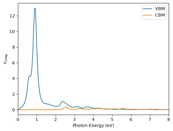

From the dielectric function above we see that this particular defect (the Ga vacancy in the neutral q=0 state) is much better at capturing electrons from the valence band via dipole transitions than it is at emitting electrons to the conduction band via dipole transitions.

Of course for a complete picture of photoconductivity, the Frank-Condon type of vibrational state transition should also be considered, but we are already pushing the limits of what is acceptable in the independent-particle picture so we will leave that for another time.

Dipole Matrix Elements¶

We can also check the dipole matrix elements for the (VBM)→(defect) and (defect)→(CBM) transitions explicitly by calling the plot_optical_transitions method as shown below. The function returns a summary pandas.DataFrame object with the dipole matrix elements as well as the ListedColormap and Normalize objects for plotting the color bar. These objects can then be passed to other instances of the plotting function to ensure that the color bar is consistent.

import matplotlib as mpl
from pymatgen.analysis.defects.plotting.optics import plot_optical_transitions

fig, ax = plt.subplots()
cm_ax = fig.add_axes([0.8, 0.1, 0.02, 0.8])
df_k0, cmap, norm = plot_optical_transitions(
    hd0, kpt_index=1, band_window=5, x0=3, ax=ax
)
df_k1, _, _ = plot_optical_transitions(
    hd0, kpt_index=0, band_window=5, x0=0, ax=ax, cmap=cmap, norm=norm
)
mpl.colorbar.ColorbarBase(cm_ax, cmap=cmap, norm=norm, orientation="vertical")
ax.set_ylabel("Energy (eV)")
ax.set_xticks([0, 3])
ax.set_xticklabels(["Kpoint-0", "Kpoint-1"])

[Text(0, 0, 'Kpoint-0'), Text(3, 0, 'Kpoint-1')]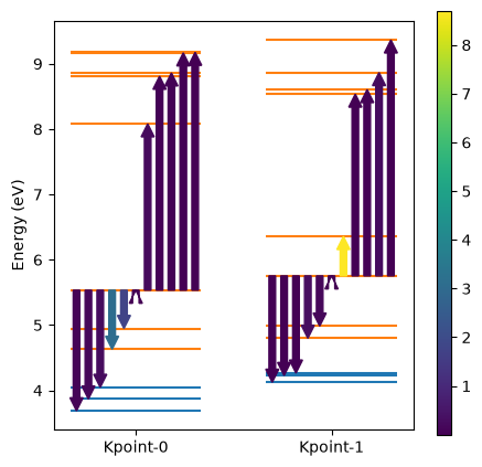

The DataFrame object containing the dipole matrix elements can also be examined directly.

df_k0